LCS Reprocessed
| Dataset Name | Sensor | Make | Spatial Resolution | Temporal Resolution | Start Date | End Date |
|---|---|---|---|---|---|---|
| LCS Reprocessed |  |
Observation | 0.04° X 0.04° | Daily | 2016-01-01 | 2018-05-27 |
Dataset Description
Reprocessed LCS (Lagrangian Coherent Structures) are a daily-global altimetry-derived and gridded product calculating Finite-Time Lyapunov Exponents (FTLE). It characterizes the transport properties of the ocean surface currents from a Lagrangian frame of reference.
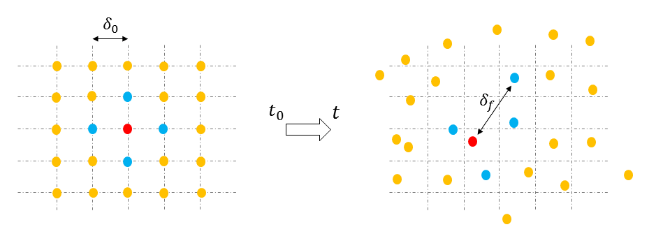
A grid of passive tracers (hypothetical massless particles) is initialized over the global domain with an initial uniform spacing of 4 km x 4 km. A flow map is then approximated by integrating particle trajectories for a fix period of time, (tau=15) days. At its fundamental levels, local Lyapunov exponents provide a metric for exponential rate of divergence for a pair of adjacent tracers:
such that \(\Lambda\) is the Lyapunov exponent, and \(\delta x(t)\), \(\delta x(0)\) represent the separation between the tracers at times \(t\) and \(t_0\), receptively.
After integrating the particles for the fixed period of time, (tau=15), FTLE fields are computed to demonstrate the local dispersion as well as local displacements (see example figures below). The particles can be integrated either forward or backward in time. The local maxima of the FTLE scalar field (ridges) can be interpreted as stable and unstable manifolds of the flow field in the case of forward and backward integration, respectively.
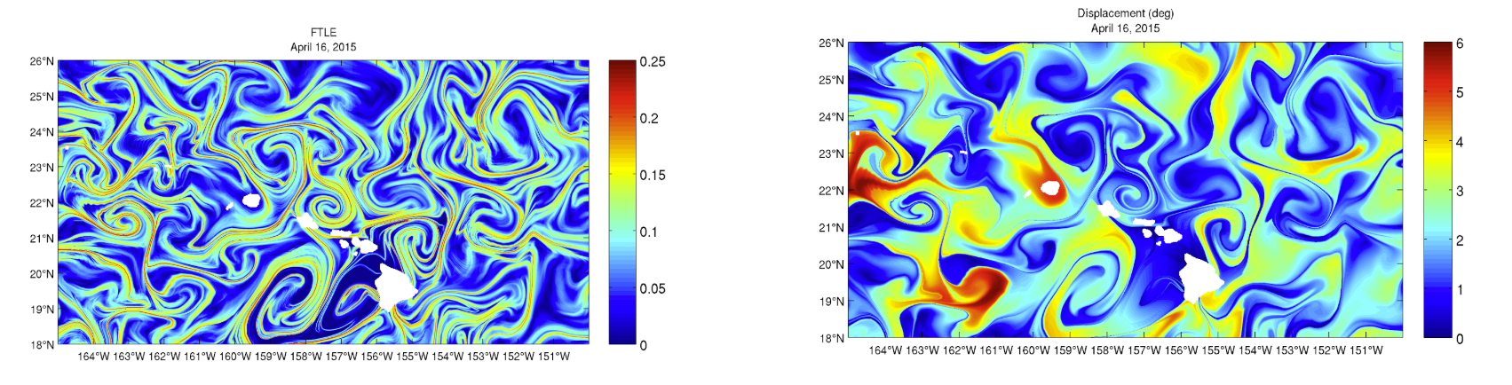
Please refer to the documentation below for more detailed information regarding FTLE mathematical framework.
Table of Variables
Data Source
Simons CMAP
https://github.com/mdashkezari/opedia/tree/master/CS
https://github.com/mdashkezari/opedia/tree/master/CS/docs/CS.pdf